Common signal representations

Many problems in signal and image processing consist in estimating a signal of interest from noisy and/or incomplete measurements. Such problems can be addressed by exploiting characteristics or regularities of natural signal and images, which can be identified or highlighted using specific signal representations. In this applied course, we will discuss the commonly used signal and image representations.

%load_ext autoreload
%autoreload 2

The autoreload extension is already loaded. To reload it, use:
  %reload_ext autoreload

Basics

Signal

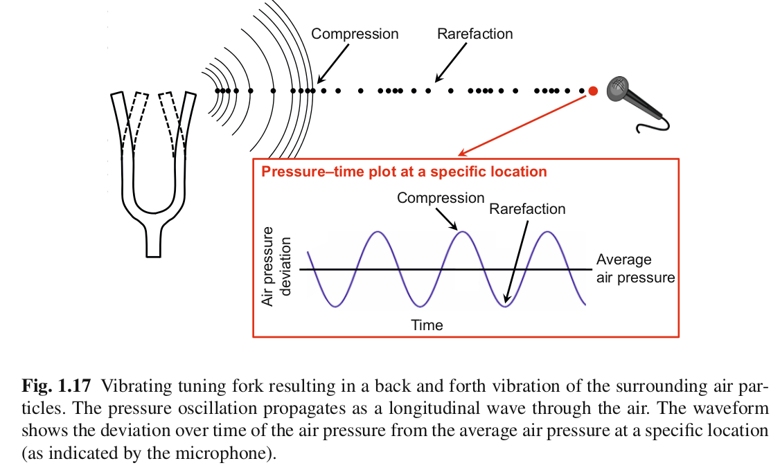
Signal processing starts with a sensor that acquires an analog signal characterizing a physical phenomenon. For instance, a microphone converts an acoustic wave into an electric signal.

Image credit: Meinard Müller, “Fundamentals of Music Processing”, Springer 2015

Digital signal

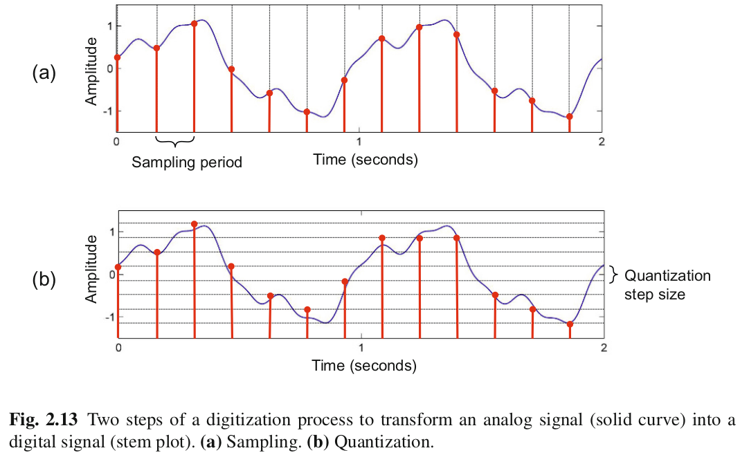
For diginal processing, the signal is sampled and quantized.

Image credit: Meinard Müller, “Fundamentals of Music Processing”, Springer 2015

Below, we import the library soundfile (as sf), and read the information of the bird-thrush-nightingale-03.wav file located in the audio folder using the sf.info function. If you want to know more about this function, just run sf.info? in a code cell.

import soundfile as sf 
wavfile = 'audio/bird-thrush-nightingale-03.wav'
info = sf.info(wavfile)
print(info)

audio/bird-thrush-nightingale-03.wav
samplerate: 44100 Hz
channels: 1
duration: 5.490 s
format: WAV (Microsoft) [WAV]
subtype: Signed 16 bit PCM [PCM_16]

We can also use the IPython package to listen to this audio signal.

import IPython
IPython.display.Audio(wavfile)

Question: Using the variable info, compute the number of samples in this audio signal. You will verify your answer by loading the audio signal using the sf.read function of soundfile.

Answer: The number of samples is given by the duration of the signal (in seconds) multiplied by the sample rate (in Hz).

print(int(info.samplerate*info.duration))

x, sr = sf.read(wavfile)
print(x.shape[0])

242119
242119

The above information tells us that this file is a WAV file using a 16-bit pulse-code modulation (PCM) representation. In particular, it means that the signal is quantized using 16 bits per sample. The amplitude of the signal is therefore represented using $2^{16} = 65 536$ values.

Representations of signals in the discrete time and frequency domains

Time-domain representation

To develop models and algorithms in signal processing we need to work with mathematical notations or representations of the physical signals we acquire in the real world.

Let's start with the most simple representation in the time domain. We denote by $x(t) \in \mathbb{R}$ a signal whose samples are real valued and which is defined in the discrete-time domain $t \in \mathbb{Z}$.

In signal processing, we can define different classes of signals, which allows us to define different transformations of the signals. For instance, we can assume that the sum of the absolute value of the signal samples is finite, i.e., $\sum\limits_{t \in \mathbb{Z}} |x(t)| < \infty.$ This assumption allows us to define the discete-time Fourier transform (DTFT). Understanding the DTFT first is useful to understand a more practical transform called the discrete Fourier transform (DFT) (spoiler: The DFT is a sampled version of the DTFT). But our goal is not to create signal processing heroes in this course, so we will directly jump to the DFT. Don't be too disapointed though, you can have a look at the appendices to learn about the DTFT and its relation with the DFT.

Real-world signals

So let's consider a really practical situation, where we acquire signals during a limited period of time and using sensors with limited dynamics. This implies that the signals are of finite length, amplitude, and energy. We therefore always have:

• $ x(t) \neq 0$ only for $t \in \{0,...,T-1 \}$, this set being called the time support of the signal;

• $ \sum\limits_{t \in \mathbb{Z}} |x(t)| = \sum\limits_{t=0}^{T-1} |x(t)| < \infty$.

We can therefore also represent a signal as a vector $\mathbf{x} \in \mathbb{R}^T$, where the entry of index $t \in \{0,...,T-1 \}$ contains the sample $x(t)$.

Question: Aren't you puzzled by some incoherence between what we've seen before about digital signals and this mathematical representation of supposedly real-world signal? In 1976, a British statistician named George Box wrote “All models are wrong, some are useful.” The above model of real-world signals is wrong, but definitely useful in so many daily-life applications.

Answer: The amplitude is quantized and not real valued.

The waveform

So, a signal is actually a function from the discrete-time domain to the amplitude domain: $x : \mathbb{Z} \mapsto \mathbb{R}$, or if you prefer $x : \{0,...,T-1\} \mapsto \mathbb{R}$. Can we look at the graph of this function? Of course we can, and this is called the waveform.

For audio signals, the waveform represents the deviation over time of the air pressure (with respect of the average air pressure) at the microphone location, it's a pressure-time plot. Let's look at the waveform of our bird recording.

import matplotlib.pyplot as plt
import numpy as np
fontsize = 13

x, sr = sf.read(wavfile)
T = x.shape[0]

time_axis = np.arange(T)/sr

plt.figure(figsize=(10,4))
plt.plot(time_axis, x)
plt.xlabel('time (s)', fontsize=fontsize)
plt.ylabel('amplitude', fontsize=fontsize)
plt.title('waveform', fontsize=fontsize)

Text(0.5, 1.0, 'waveform')

Question: Why is the signal centered around 0? What pressure does this amplitude correspond to?

Answer: The audio signal results from the vibration of a physical system, which causes oscillations of the surrounding air particles. These should eventually go back to their equilibrium position, corresponding to the average air pressure.

Let's look at another, maybe simpler signal. In the next cell we load an electrocardiogram (ECG) and plot the corresponding waveform. Electrocardiography is a method to record heart activity by using electrodes to measure electrical changes on the skin. An ECG thus corresponds to the recording of a heart's electrical activity, and the waveform is a voltage-time plot.

from utils import load_ecg

x, sr = load_ecg()
T = x.shape[0]
time_axis = np.arange(T)/sr

plt.figure(figsize=(10,4))
plt.plot(time_axis, x)
plt.xlabel('time (s)', fontsize=fontsize)
plt.ylabel('amplitude', fontsize=fontsize)
plt.title('waveform', fontsize=fontsize)

Text(0.5, 1.0, 'waveform')

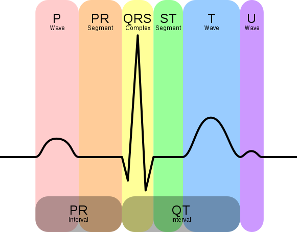
The image below shows a schematic representation of a normal ECG. According to Wikipedia, normal rhythm produces four entities – a P wave, a QRS complex, a T wave, and a U wave – that each have a fairly unique pattern.

• The P wave represents atrial depolarization.
• The QRS complex represents ventricular depolarization.
• The T wave represents ventricular repolarization.
• The U wave represents papillary muscle repolarization.

Image credit: Wikipedia.

An ECG captures multiple repetitions of this pattern, corresponding to several cardiac cycles. Unfortunately, the real ECG is quite different from this schematic representation, as it contains other periodic components that make it difficult to visualize the above patterns. Decomposing the signal in different components associated with different frequencies is very useful to remove such perturbations. This decomposition is achieved using the discrete Fourier transform (DFT).

Frequency domain representation

Discrete Fourier transform (DFT)

Let $x(t) \in \mathbb{R}$ be a signal of finite support $ \{ 0,...,T-1 \} $. The discrete Fourier transform (DFT) of order $F \in \mathbb{N}$ is defined by:

$$ X(f) = \sum\limits_{t=0}^{T-1} x(t) \exp\left(-j 2 \pi \frac{f t}{F}\right), \qquad f \in \{0,...,F-1\}.$$

If $F > T$, the signal is zero-padded and if $F < T$ it is truncated. In other words, we artificially change the length $T$ of the signal so that in the end it is equal to the DFT order $F$.

The inverse DFT is defined by:

$$ x(t) = \frac{1}{F} \sum\limits_{f=0}^{F-1} X(f) \exp\left(+j 2 \pi \frac{f t}{F}\right), \qquad t \in \mathbb{Z}. $$

Alternatively but equivalently, we could define the DFT by normalizing both the direct and the inverse transforms by $\frac{1}{\sqrt{F}}$, instead of normalizing the inverse DFT by $\frac{1}{F}$.

For real-valued signals, the DFT is complex valued, it gives the spectrum of the signal. So we will generally look at the modulus of the DFT, which is called the magnitude spectrum, or the squared modulus, which is called the power spectrum. The argument of the DFT is called the phase spectrum.

Hermitian symmetry

Let's have a look at the magnitude and power spectrum of our ECG signal.

F = T # number of points for the DFT

x_dft = np.fft.fft(x, F) # DFT

freq_axis = np.arange(F)/F*sr # frequency axis in Hertz

plt.figure(figsize=(10,3))
plt.plot(freq_axis, np.abs(x_dft))
plt.title('Magnitude spectrum')
plt.xlabel('frequency (Hz)')

plt.figure(figsize=(10,3))
plt.plot(freq_axis, 10*np.log10(np.abs(x_dft)**2))
plt.title('Power spectrum in dB')
plt.xlabel('frequency (Hz)')

Text(0.5, 0, 'frequency (Hz)')

We observe in the above spectra a form of symmetry around the middle of the frequency axis. This comes from an important property of the DFT of real-valued signals, which is called the Hermitian symmetry and is defined by:

$$X(F-f) = X^*(f), \qquad f \in \{0,...,F-1\},$$

where $\cdot^*$ denotes the complex conjugate.

Let's print the values of the DFT at the zero frequency ($f=0$) and at the Nyquist frequency ($f= F//2$), assuming that $F$ is even.

# zero-frequency coefficient
x_dft_0 = x_dft[0]
print("DFT coef. at frequency 0: ", end='')
print(x_dft_0)

# Nyquist-frequency coefficient
x_dft_nyq = x_dft[F//2]
print("DFT coef. at Nyquist frequency: ", end='')
print(x_dft_nyq)

DFT coef. at frequency 0: (642.9717821672234+0j)
DFT coef. at Nyquist frequency: (0.43257941181657067+0j)

We observe that the DFT coefficients at the zero and Nyquist frequencies are real-valued, i.e., the imaginary part is exactly zero. This can be easily verified theoretically as follows:

• $X(F-F/2) = X(F/2) = X^*(F/2) \in \mathbb{R}$, using the Hermitian symmetry property;
• $X(0) = \sum_{t=0}^{T-1} x(t) \in \mathbb{R}$, using the definition of the DFT.

The DFT can consequently be splitted into 4 parts:

1. The zero-frequency coefficient $X(0)$, which is real valued;
2. The (F/2-1) coefficients $X(f)$ for $f = 1,...,F/2-1$, which are sometimes called the positive frequencies;
3. The Nyquist-frequency coefficient $X(F/2)$, which is real valued;
4. The (F/2-1) coefficients $X(f)$ for $f = F/2+1,...,F-1$, which are sometimes called the negative frequencies.

The Hermitian symmetry property tells us that the negative-frequency coefficients are equal to the conjugate of the positive-frequency coefficients when we reverse the frequency axis. Let's verify this.

# positive-frequency coefficient
x_dft_p = x_dft[1:F//2] # shape F/2-1

# negative-frequency coefficient
x_dft_n = x_dft[F//2+1:] # shape F/2-1

# using the Hermitian symetry property, we can predict the negative part from the positive one
x_dft_n_from_p = np.conj(np.flipud(x_dft_p))

# we can verify that Hermitian symmetry holds
print("Error: ", end='')
print(np.sum(x_dft_n - x_dft_n_from_p))

Error: (-1.511325786740514e-13-8.638922910364499e-14j)

Wow, this was harsh signal processing stuff. Don't worry, what you simply need to remember is the following:

Real-valued signals have an Hermitian symmetric spectrum, so we usually only keep the non-redundant part of the spectrum, up to the Nyquist frequency, here we go.

x_dft = x_dft[:F//2+1] # only keep the positive frequencies (including zero and Nyquist freq.)
freq_axis = freq_axis[:F//2+1]

plt.figure(figsize=(10,5))
plt.plot(freq_axis, 10*np.log10(np.abs(x_dft)**2))
plt.title('Power spectrum in dB')
plt.xlabel('frequency (Hz)')

Text(0.5, 0, 'frequency (Hz)')

We see that in this signal, most of the energy is concentrated in the low frequency, so let's zoom in a bit more. We plot again the waveform for discussion.

plt.figure(figsize=(10,5))
plt.plot(freq_axis, 10*np.log10(np.abs(x_dft)**2))
plt.title('Power spectrum in dB')
plt.xlabel('frequency (Hz)')
plt.xlim((0,60))

plt.figure(figsize=(10,4))
plt.plot(time_axis, x)
plt.xlabel('time (s)', fontsize=fontsize)
plt.ylabel('amplitude', fontsize=fontsize)
plt.title('waveform', fontsize=fontsize)

Text(0.5, 1.0, 'waveform')

Notice that we have a difference of about 60 dB between the most and least energetic frequency components of this signal. When we divide the amplitude of a signal by 2, we loose $20 \log_{10}(2) = 6$ dB, so a 60 dB decrease is quite significant.

Filtering of an ECG signal

We can make other observations from this power spectrum:

• The spectrum includes very low but strong frequency components, which correspond to the slowly-varying fluctuations in the waveform. These are typically caused by motion of the recording device or the patient, or by breathing.
• In addition, the spectrum reveals a strong component at 50 Hz. This is caused by interference from the power grid, which transmits electricity exactly at that frequency.

In order to use the ECG for diagnosis, we would like to eliminate these frequency components, since they are not associated to heart activity. This is a filtering task in signal processing. The naive approach would simply consist in zeroing the DFT coefficients at the frequencies we want to discard, and reconstructing the time-domain signal by inverse DFT.

Exercise: Complete the cell below to implement this naive filtering approach.

# from utils import freq2index, recon_hermitian_symmetry_2

# # high-pass filtering
# ind_freq_HP = freq2index(?, sr, F) # cut-off freq. index of the high-pass filter
# x_dft[?] = ?

# # band-stop filtering
# ind_freq_BS = freq2index(?, sr, F) # center freq. index of the band-stop filter
# x_dft[?] = ?

# # reconstruct full spectrum using Hermitian symmetry
# x_dft_full = recon_hermitian_symmetry(x_dft)

# # reconstruct time domain signal with inverse DFT
# x_filt = np.real(np.fft.ifft(x_dft_full))

Solution

from utils import freq2index, recon_hermitian_symmetry

# high-pass filtering
ind_freq_HP = freq2index(2, sr, F) # cut-off freq. index of the high-pass filter
x_dft[:ind_freq_HP] = 0

# band-stop filtering
ind_freq_BS = freq2index(50, sr, F) # center freq. index of the band-stop filter
x_dft[ind_freq_BS-2:ind_freq_BS+2] = 0

# reconstruct full spectrum using Hermitian symmetry
x_dft_full = recon_hermitian_symmetry(x_dft)

# reconstruct time domain signal with inverse DFT
x_filt = np.real(np.fft.ifft(x_dft_full))

Let's plot the results, what do you observe?

plt.figure(figsize=(10,4))
plt.plot(time_axis, x)
plt.xlabel('time (s)', fontsize=fontsize)
plt.ylabel('amplitude', fontsize=fontsize)
plt.title('waveform', fontsize=fontsize)

plt.figure(figsize=(10,4))
plt.plot(time_axis, x_filt)
plt.xlabel('time (s)', fontsize=fontsize)
plt.ylabel('amplitude', fontsize=fontsize)
plt.title('filtered waveform', fontsize=fontsize)

plt.figure(figsize=(10,4))
plt.plot(time_axis, x_filt)
plt.xlabel('time (s)', fontsize=fontsize)
plt.ylabel('amplitude', fontsize=fontsize)
plt.title('filtered waveform', fontsize=fontsize)
plt.xlim((3.2,4.0))

(3.2, 4.0)

This simple brick-wall filter is known to cause ringing artifacts in the reconstructed time domain signal. You should probably ask a real signal processing hero to help you in the filter design, which is out of the scope of this course.

Geometric interpretation and alternatives to the DFT

To finish this part, let's discuss about a geometric interpretation of the DFT. This is probably what you should really remember about the DFT, because it shares strong connections with other aspects of signal representations that will be discussed in following lessons.

Let $\mathbf{x} \in \mathbb{R}^T$ be the vector representation of the signal $x(t)$, $t \in \{ 0,...,T-1 \}$, and let $\mathbf{u}_f \in \mathbb{C}^T$ be the vector of entries $\mathbf{u}_f(t) = \frac{1}{\sqrt{F}} \exp\left(+j 2 \pi \frac{f t}{F}\right)$, $t \in \{ 0,...,T-1 \}$. This vector can be regarded as a complex sinusoid of frequency $f/F$, using Euler's formula:

$$ e^{+j 2 \pi \frac{f t}{F}} = \cos\left( 2 \pi \frac{f t}{F} \right) + j \sin\left( 2 \pi \frac{f t}{F} \right). $$

Then the (normalized) DFT can be expressed as inner products (on the complex vector space $\mathbb{C}^T$) between the signal $\mathbf{x}$ and complex sinusoids $\mathbf{u}_f$ of different frequencies:

$$ X(f) = \langle \mathbf{x}, \mathbf{u}_f \rangle = \mathbf{u}_f^H \mathbf{x}, \qquad f \in \{0,...,F-1\}, $$

where $\cdot^H$ denotes Hermitian transpose (transpose + complex conjugate).

If we assume that $F = T$ (after zero-padding or truncation), the vector $\check{\mathbf{x}} \in \mathbb{C}^F$ of DFT coefficients is obtained by multiplying the signal $\mathbf{x} \in \mathbb{R}^T$ with the DFT matrix $\mathbf{U} \in \mathbb{C}^{F \times T}$ where each row of index $f \in \{0,...,F-1\}$ is defined by ${\mathbf{u}_f^H \in \mathbb{C}^T}$:

$$ \check{\mathbf{x}} = \mathbf{U} \mathbf{x}, \qquad (\mathbf{U})_{f,:} = \mathbf{u}_f^H. $$

The figure below shows the real (left) and imaginary (right) parts of the DFT matrix:

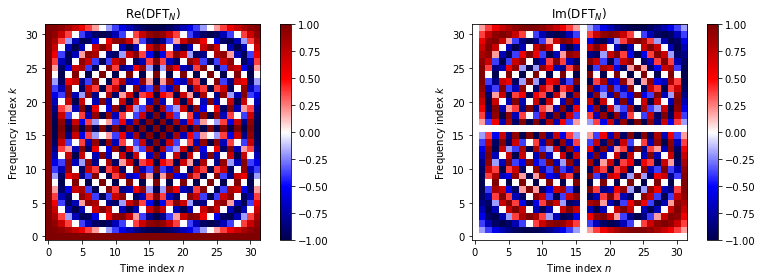
Image credit: Meinard Müller, “Fundamentals of Music Processing”, Springer 2015

Question: Can you explain why we observe white horizontal lines on the right figure?

Answer: These correspond to the zero and Nyquist frequencies, see discussion above.

Now let's focus on the inverse DFT. If we go back to its definition (in the normalized case):

$$ x(t) = \frac{1}{\sqrt{F}} \sum\limits_{f=0}^{F-1} X(f) \exp\left(+j 2 \pi \frac{f t}{F}\right), \qquad t \in \mathbb{Z}, $$

we see that the time-domain signal is represented as a linear combination of complex sinusoids. How come this operation can lead to a real-valued time-domain signal? Well, this is precisely due to the Hermitian symmetry property of the DFT of real-valued signals.

Finally, it can be shown that the unit-norm vectors $\{\mathbf{u}_f \in \mathbb{C}^T\}_{f=0}^{F-1}$ are orthogonal and span $\mathbb{C}^T$, so they form an othonormal basis of $\mathbb{C}^T$ and the DFT is just a change of basis. The DFT matrix is therefore unitary and we have

$$ \mathbf{U}^H \hat{\mathbf{x}} = \mathbf{U}^H \mathbf{U} \mathbf{x} = \mathbf{x}.$$

In summary, the DFT gives us the decomposition of the time-domain signal onto the set of complex sinusoids $\{\mathbf{u}_f, f \in \{0,...,F-1\}\}$, and the inverse DFT reconstructs the time-domain signal as a linear combination of the same complex sinusoids, weighted by the DFT coefficients: $$ \mathbf{x} = \sum\limits_{f=0}^{F-1} X(f) \mathbf{u}_f = \sum\limits_{f=0}^{F-1} \langle \mathbf{x}, \mathbf{u}_f \rangle \mathbf{u}_f. $$

There exist alternatives to Fourier's complex sinusoids for spectral analysis. The above geometric interpretation remains valid, these alternatives simply consist in replacing the complex sinusoids by other functions that also form an othonormal basis of $\mathbb{C}^T$ (or $\mathbb{R}^T$). For instance, using cosine functions defined by $$ \mathbf{u}_f(t) = \sqrt{\frac{2}{T}} \cos\left[ \frac{\pi}{T} \left(f + \frac{1}{2}\right) \left(t + \frac{1}{2}\right) \right] $$ leads to the discrete cosine transform (DCT) of type IV. The DCT (or variants of the DCT) is very popular in data compression, for instance it is used in the JPEG and MP3 compression standards. We will come back to this at the end of the notebook.

In the next section, we will discuss some limitations of the DFT and how they can be addressed using time-frequency representations.

Time-frequency representation

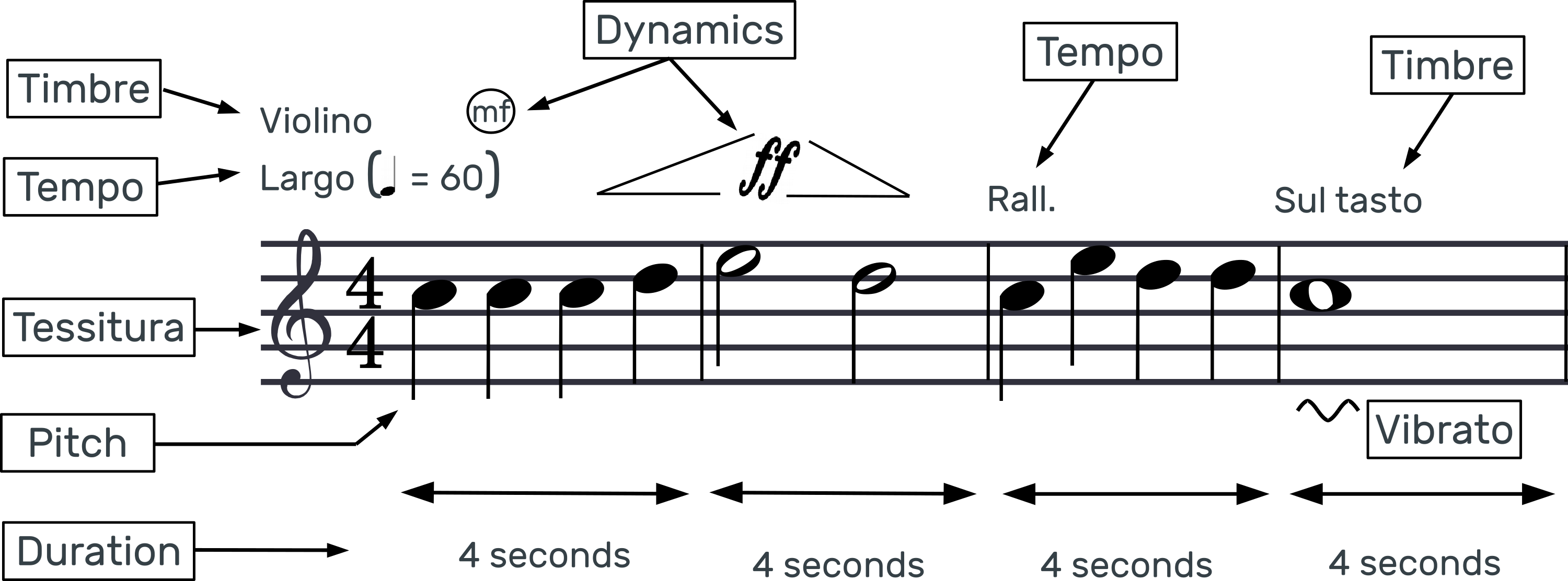
Consider the problem of automatic music transcription, i.e., estimating a musical score given an audio recording. You have below an example of musical score (with excessive information, this is for the sake of the example). A musical score is used by musicians to indicate a succession of audio events (notes) with indicators of pitch, dynamics, tempo, and timbre. Tempo and rhythm relate to time (measured in seconds), pitch and timbre relate to frequency (measured in Hertz), dynamics relates to intensity or power (measured in decibels).

Let's consider a piano recording of "Au clair de la lune" (the melody corresponding to the above musical score) and plot the signal representations that we are familiar with, the waveform and the power spectrum.

IPython.display.Audio('audio/acdll.wav')

x, fs = sf.read('audio/acdll.wav')
x = x/np.max(x)

T = x.shape[0]
f = np.arange(T)*fs/T
t = np.arange(T)/fs

plt.figure(figsize=(10,3))

plt.plot(t, x)
plt.title('Waveform')
plt.xlabel('Time (s)')
plt.ylabel('Amplitude')

x_dft = np.fft.fft(x)

plt.figure(figsize=(10,3))
plt.plot(f[:int(T/2)], 20*np.log10(np.abs(x_dft[:int(T/2)])))
plt.title('Power spectrum')
plt.xlabel('Frequency (Hz)')
plt.ylabel('Magnitude in dB')

Text(0, 0.5, 'Magnitude in dB')

Question: In order to solve our automatic music transcription task, we would like to compute a representation that highlights the characteristics of the signal along the same dimensions as in the musical score. Explain what is missing the waveform and power spectrum representations.

Answer:

In the waveform, the frequency information is missing. In the power spetrum, the frequency information is "averaged" over the entire time domain, such that local phenomena (individual musical notes here) become global in the DFT.

Fourier analysis is insufficient when the frequency characteristics of the signal vary with time. We speak of non-stationarity. The non-stationarity can be slow, for instance in the case of a vibrato in music, where the frequency characteristics of the sound (notably its pitch) slowly vary with time. Or it can be fast, for instance in the case of a percussive or more generally transient sound.

To compute a representation that highlights the characteristics of the signal along time, frequency, and intensity, we need a local DFT. This is called the short-time Fourier transform (STFT) and leads to a representation called the spectrogram.

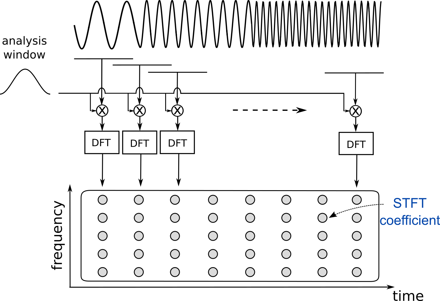
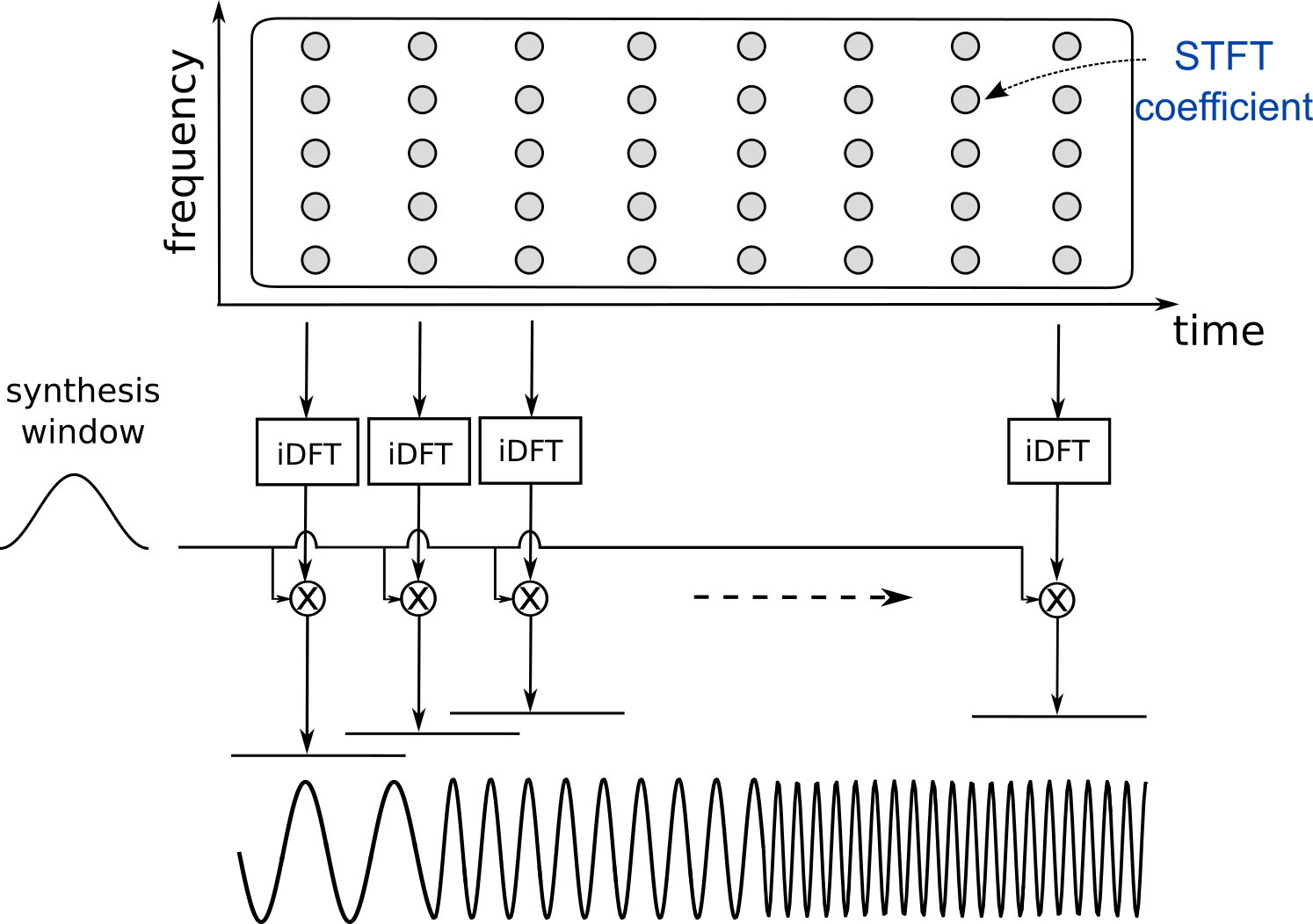
The short-time Fourier transform (STFT) is obtained by computing the discrete Fourier transform (DFT) on short overlapping smoothed windows of the signal, as illustrated below.

We are going to define the STFT properly.

Windowing

Let $x(t) \in \mathbb{R}$ be a signal defined in the time domain $t \in \mathbb{Z}$. A frame of the signal is defined for all $n \in \mathbb{Z}$ by:

$$ x_n(t) = x(t + nH) w_a(t),$$

where

• $w_a(t)$ is an analysis window of time support $\{0,...,L-1\}$;
• $H$ is the analysis hop size (increment) with $L/H \in \mathbb{N}$;
• the overlap between two successive frames is equal to $L_w - H$.

$x(t + nH)$ is a shifted version of $x(t)$, where the shift is equal to $n$ times the analysis hop size $H$.

Question: Assume $x(t) \neq 0$ only for $0 \le t \le T-1 $, what is the time support of $x(t + nH)$? If $n > 0$, is the signal shifted left or right?

Answer: $x(t + nH) \neq 0$ for $0 \le t + nH \le T-1 \Leftrightarrow - nH \le t \le T-1 - nH$. If $n > 0$ the signal is shifted left.

The time support of the frame $x_n(t)$ is the same as that of the analysis window $w_a(t)$. In audio signal processing, we typically choose a short analysis window (between 10 and 100 ms) to assume the stationarity of the signal over its time support, we speak of local stationarity.

Remark: In the above definition of the STFT, we shift the signal $x(t)$ by a number of samples $nH$ instead of shifting the analysis window $w_a(t)$ as it is represented in the above figure. This definition corresponds to the band-pass convention. There exist another definition, in the low-pass convention, where the analysis window is shifted.

Direct STFT

The STFT is defined for all time-frequency points $(f,n) \in \{0,...,F-1\} \times \mathbb{Z}$ by the DFT of the frame $x_n(t)$:

$$ X(f,n) = \sum_{t \in \mathbb{Z}} x_n(t) \exp\left(-j2\pi \frac{ft}{F}\right),$$

where $F$ is the order of the DFT, which can be chosen as $F=L$. The STFT inherits the properties of the DFT; it is complex valued and the STFT of a real-valued signal exhibits the Hermitian symmetry. Thus, as for the DFT, we usually only keep the non-redundant part of the spectrum.

In practice, the time support of the STFT is finite (because the time-domain signal is of finite length $T$), such that we can denote by $\mathbf{X} \in \mathbb{C}^{F \times N}$ the STFT matrix where $F$ is the number of frequency bins and $N$ the number of time frames (which can be computed from the $T$, $L$ and $H$). Then,

• the modulus of the STFT $|\mathbf{X}| \in \mathbb{R}_+^{F \times N}$ is called the magnitude spectrogram;

• the squared modulus $|\mathbf{X}|^{\odot 2} \in \mathbb{R}_+^{F \times N}$ of the STFT is called the power spectrogram, we generally compute the power spectrogram in dB: $10 \log_{10}|\mathbf{X}|^{\odot 2} = 20 \log_{10}|\mathbf{X}|$;

• the argument $\arg(\mathbf{X}) \in [0, 2\pi[^{F \times N}$ of the STFT is called the phase spectrogram.

We are going to implement the STFT using the sine window, which is actually the square root of the Hann window (there exist many different windows with different properties):

$$ w_a(t) = \sin\left( \frac{\pi}{L} \left(t + \frac{1}{2}\right) \right), \qquad t = 0,..., L-1. $$

Read the code in the following cells to understand how the STFT is computed.

fs = 16000 # sampling rate
wlen_sec = 32e-3 # STFT window length in seconds
hop_percent = 0.5  # hop size as a percentage of the window length
L = wlen_sec*fs # window length in samples
L = int(np.power(2, np.ceil(np.log2(L)))) # round to the next power of 2 to fasten fft 
H = int(hop_percent*L) # hop size in samples
n_fft = L # number of points (i.e. order) of the discrete Fourier transform
n_bins = L//2 + 1  # number of positive frequency bins

win = np.sin(np.arange(.5,L-.5+1)/L*np.pi); # sine analysis window
time_axis = np.arange(0, L)/fs
plt.plot(time_axis, win)
plt.xlabel('time (s)')
plt.ylabel('amplitude')
plt.title('sine window')

Text(0.5, 1.0, 'sine window')

from utils import preprocessing_stft

x = preprocessing_stft(x, L, H) # some preprocessing to deal with edges and ensure perfect reconstruction (you do not need to understand this for the moment)
T = x.shape[0] # signal length
n_frames = int( (T-L)/H ) + 1 # number of time frames

X = np.zeros( (n_bins, n_frames), dtype=np.cfloat ) # STFT matrix

#### STFT computation ####
for n in np.arange(n_frames):
    beg_frame = n*H
    end_frame = beg_frame + L
    x_n = x[beg_frame:end_frame]*win
    X_n = np.fft.fft(x_n)
    X[:,n] = X_n[:n_bins]

Below, we display the resulting power spectrogram.

X2_dB = 10*np.log10(np.abs(X)**2 + 1e-10) # power spectrogram in dB

plt.figure(figsize=(10,7))
plt.imshow(X2_dB, origin='lower',  aspect='auto', cmap='magma', extent=[0, (n_frames-1)*H/fs, 0, fs/2])

plt.clim(vmin=-50, vmax=None)
plt.colorbar()   
plt.xlabel('time (s)')
plt.ylabel('frequency (Hz)')
plt.title('power spectrogram')

Text(0.5, 1.0, 'power spectrogram')

Question: Explain what you observe in this spectrogram representation by comparing it with the corresponding musical score. Propose a simple method to estimate the musical score from this representation.

Answer: We observe the succession of musical notes. For instance, we see that the audio recording starts with three repetitions of the same note. Indeed, a note is characterized by its fundamental frequency (also called the pitch), which corresponds to the frequency of the first peak in its spectrum. We could therefore estimate the musical score by peak picking from the spectrogram representation.

Inverse STFT and overlap-add

The inverse STFT is computed by taking the inverse DFT of the spectra at all time indices and by a procedure called overlap-add.

For each time frame $n \in \mathbb{Z}$ of the STFT, we first compute the inverse DFT:

$$ \hat{x}_n(t) = \frac{1}{F}\sum_{f=0}^{F-1} X(f,n) \exp\left(+ j2\pi \frac{ft}{F}\right).$$

The inverse STFT is then computed by overlap-add, for all $t \in \mathbb{Z}$:

$$ \hat{x}(t) = \sum_{n \in \mathbb{Z} } w_s(t-nH) \hat{x}_n(t-nH),$$

where $w_s(t)$ is a smooth synthesis window with the same support as the analysis window.

Read the following cells that implement the inverse STFT.

x_rec = np.zeros((n_frames-1)*H + L)

X_n_complete = np.zeros(L, dtype=np.cfloat)

#### Inverse STFT computation ####
for n in np.arange(n_frames):
    X_n_complete = recon_hermitian_symmetry(X[:,n])
    x_n_rec = np.real(np.fft.ifft(X_n_complete))
    ind_beg = n*H
    ind_end = ind_beg+L
    x_rec[ind_beg:ind_end] += x_n_rec*win

Question: Plot the difference between the original audio signal and its reconstruction after direct and inverse STFT, what do you conclude?

Answer: The amplitude of the error is about 1e-16, indicating that the reconstruction is perfect.

plt.plot(x-x_rec)

[<matplotlib.lines.Line2D at 0x7fe0d2515f70>]

Perfect reconstruction

We can show that perfect reconstruction is achieved, i.e., $\hat{x}(t) = x(t)$ for all $t \in \mathbb{Z}$, if the analysis and synthesis windows satisfy:

$$ \sum_{n \in \mathbb{Z} } w_a(t-nH)w_s(t-nH) = 1.$$

Hint for the proof (only for the brave): $\displaystyle \frac{1}{F} \sum_{f=0}^{F-1} \exp\left( -j 2 \pi \frac{ft}{F} \right) = 1$ if $t=0$, and $0$ if $t \in \mathbb{Z}^*$. It corresponds to the sum of the $F$-th roots of unity, and this result can be shown by recognizing a sum of the successive terms of a geometric sequence.

This condition is satisfied for the sine window we have used for both analysis and synthesis ($w_a(t) = w_s(t)$) and with a 50% overlap ($H = L/2$). We are going to verify this by defining an arbitrary number of time frames $N = 10$ for the overlap-add operation, such that $n=0,...,N-1$, and by computing the overlap-add operation in the last equation.

N = 10
ola = np.zeros((N-1)*H+L) # array to save the result of the overlap-add

for n in np.arange(N):
    ind_beg = n*H
    ind_end = ind_beg+L
    ola[ind_beg:ind_end] += win**2
    
plt.plot(ola)
plt.title('overlap-add of the sine window with 50% overlap')

Text(0.5, 1.0, 'overlap-add of the sine window with 50% overlap')

We indeed observe that except for the edges, the perfect reconstruction condition is verified. In practice, when computing the STFT, we will do some preprocessing (add zeros) to deal with edges. When computing the inverse STFT, we will apply the corresponding postprocessing (remove first and last coefficients) to ensure perfect reconstruction. Note that we could also simply divide by the overlap-add of the sine window after computing the inverse STFT.

Effect of the analysis window length and time-frequency resolution

In the following we will use librosa to compute spectrograms. This is a python package for music and audio analysis.

Run the following cells to analyze and listen to the recording of a glockenspiel. In particular, we will plot the spectrogram with different lengths for the analysis window.

wavfile = 'audio/glockenspiel.wav'

IPython.display.Audio(wavfile)

import librosa
import librosa.display

x, fs = sf.read(wavfile)

T = x.shape[0]
f = np.arange(T)*fs/T
t = np.arange(T)/fs

plt.figure(figsize=(12,3))

plt.plot(t, x)
plt.xlim((t[0], t[-1]))
plt.title('Waveform')
plt.xlabel('Time (s)')
plt.ylabel('Amplitude')

wlen_sec = 64e-3 # STFT window length in seconds

for wlen_sec in [16e-3, 32e-3, 64e-3]:

    hop_percent = 0.5  # hop size as a percentage of the window length
    L = wlen_sec*fs # window length in samples
    L = int(np.power(2, np.ceil(np.log2(L)))) # round to the next power of 2 to fasten fft 
    H = int(hop_percent*L) # hop size in samples
    n_fft = 2*L # number of points (i.e. order) of the discrete Fourier transform
    win = np.sin(np.arange(.5,L-.5+1)/L*np.pi); # sine analysis window

    X = librosa.stft(x, n_fft=n_fft, hop_length=H, win_length=L, window=win)
    X_db = librosa.amplitude_to_db(np.abs(X))

    plt.figure(figsize=(15,5))
    librosa.display.specshow(X_db, x_axis='time', y_axis='linear', sr=fs, hop_length=H, cmap='magma')
    plt.colorbar()
    plt.xlabel('Time (s)')
    plt.ylabel('Frequency (Hz)')
    plt.ylim((0,10000))
    plt.title('Power spectrogram with an analysis window of length ' + str(L) + ' samples')

When a glockenspiel bar is struck with a mallet, it vibrates at a fundamental frequency while emitting a series of overtones, which are generally not harmonic (i.e., not integer multiples of the fundamental frequency).

Question: Describe the structure of the spectrogram and comment on the effect of the analysis window length.

Answer:

The spectrogram essentially consists of horizontal and vertical lines. Vertical lines correspond to the percussion of the instrument bars with a mallet, which correspond to a transient sound. Horizontal lines correspond to the vibration of the bar, which correspond to a steady sound.

As the analysis window length increases, the vertical lines become thiner and the horizontal lines become thicker. This effect characterizes the trade off between time and frequency resolution. With a short analysis window, we have a good time resolution, allowing us to precisely localize events in time (the bar being struck), but we cannot at the same time precisely localize the event in frequency (the pitch of the note). With a larger analysis window, it's the contrary, we can precisely localize the event in frequency, but not in time.

To further understand this notion of resolution, read the corresponding section in the appendix. Note also that while the time-frequency resolution is fixed with the STFT, the wavelet transform adapts automatically the time-frequency resolution. With the wavelet transform, the time resolution increases with the frequency, which corresponds to the intuition that high-frequency (i.e., rapidly-varying) signal components need a better time resolution than low-frequency (i.e., slowly-varying) ones.

Another important observation that can be made by looking at the spectrogram corresponds to the repartition of the energy. We see that the energy in this signal is strongly localized in time or frequency, and most of the time-frequency points are actually associated with the black color, which corresponds to very small values on the spectrogram. Audio signals tend to be sparse in the time-frequency domain, we will come back to this notion of sparsity later on in the course.

Interpretation as the decomposition over a set of time-frequency atoms

Remember, we've seen that the computation of the DFT of a signal can be interpreted as the signal's decomposition over a set of complex sinusoids. And the time-domain signal can be reconstructed by linearly combining the complex sinusoids.

Similarly, we can see the time-frequency analysis of a signal $\mathbf{x} \in \mathbb{R}^T$ as its decomposition over a dictionary (or a set) of time-frequency atoms $\{\boldsymbol{\psi}_{fn} \in \mathbb{C}^T\}_{(f,n) \in \{0,...,F-1\}\times \mathbb{Z}}$:

$$ X(f,n) = <\mathbf{x},\boldsymbol{\psi}_{fn}> = \boldsymbol{\psi}_{fn}^H \mathbf{x} = \sum_{t \in \mathbb{Z}} x(t) \psi_{fn}^*(t).$$

In the case of the STFT (and using the normalized definition of the DFT), the time-frequency atom $\psi_{fn}(t)$ is a temporally localized frame of the complex sinusoid at frequency $f$:

$$ \psi_{fn}(t) = \frac{1}{\sqrt{L}} w(t-nH) \exp\left(+j2\pi\frac{f(t-nH)}{L}\right).$$

Inverse STFT then consists in reconstructing the time-domain signal by linear combination of the time-frequency atoms:

$$ \hat{\mathbf{x}} = \sum_{f=0}^{F-1} \sum_{n \in \mathbb{Z}} X(f,n) \boldsymbol{\psi}_{fn} = \sum_{f=0}^{F-1} \sum_{n \in \mathbb{Z}} <\mathbf{x},\boldsymbol{\psi}_{fn}> \boldsymbol{\psi}_{fn}.$$

Using different time-frequency atoms lead to different transforms. For instance, the modified discrete cosine transform (MDCT) is a local version of the DCT-IV that uses frames of cosine functions:

$$ \psi_{fn}(t) = \frac{4}{\sqrt{L}} w(t-nH) \cos\left(\frac{2\pi}{L} \left(f+\frac{1}{2}\right) \left(t-nH+\frac{1}{2}+ \frac{L}{4}\right) \right).$$

MDCT is the most widely used lossy compression technique in audio data compression. It is employed in most modern audio coding standards, including MP3.

Beyond audio spectrograms

We have been focusing on spectrograms of audio signals, but time-frequency representations such as the spectrogram are routinely used in countless applications, such as:

• Gravitational astronomy: The spectrogram below shows a gravitational wave chirp. It was obtained from the signals of both Hanford and Livingston detectors to show the characteristic sweeping chirp. As the neutron stars came closer to each other, circling faster, they produced higher frequency gravitational waves shown by the greenish line sweeping upwards. Image credits: Caltech/MIT/LIGO Lab, https://www.ligo.caltech.edu/news/ligo20171016

  

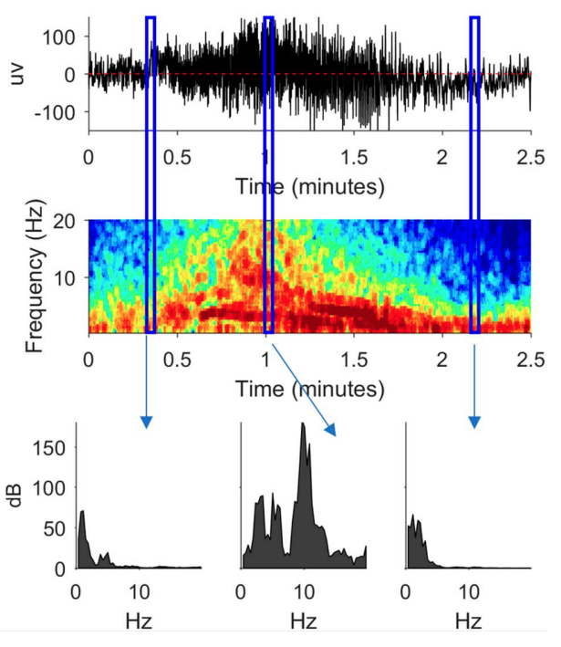
• EEG analysis: The figure below show (top) a seizure measured by EEG, (middle) with corresponding spectrograms, (bottom) and power spectra at selected times. Image credits: M.C. Ng et al., A Primer on EEG Spectrograms, Journal of Clinical Neurophysiology, 2021.

  

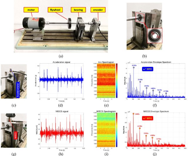
• Rotating machinery monitoring: The figure below shows (a) Rotor test bed. (b) Bearing support. (c)-(f): The time domain waveform, the spectrogram and the envelope spectrum of the signal acquired by the accelerometer. (g)-(j): The time domain waveform, the spectrogram and the envelope spectrum of the signal acquired by the MIECS. Credits: X. Xue et al., Motion induced eddy current sensor for non-intrusive vibration measurement, IEEE Sensors Journal, 2019.

  

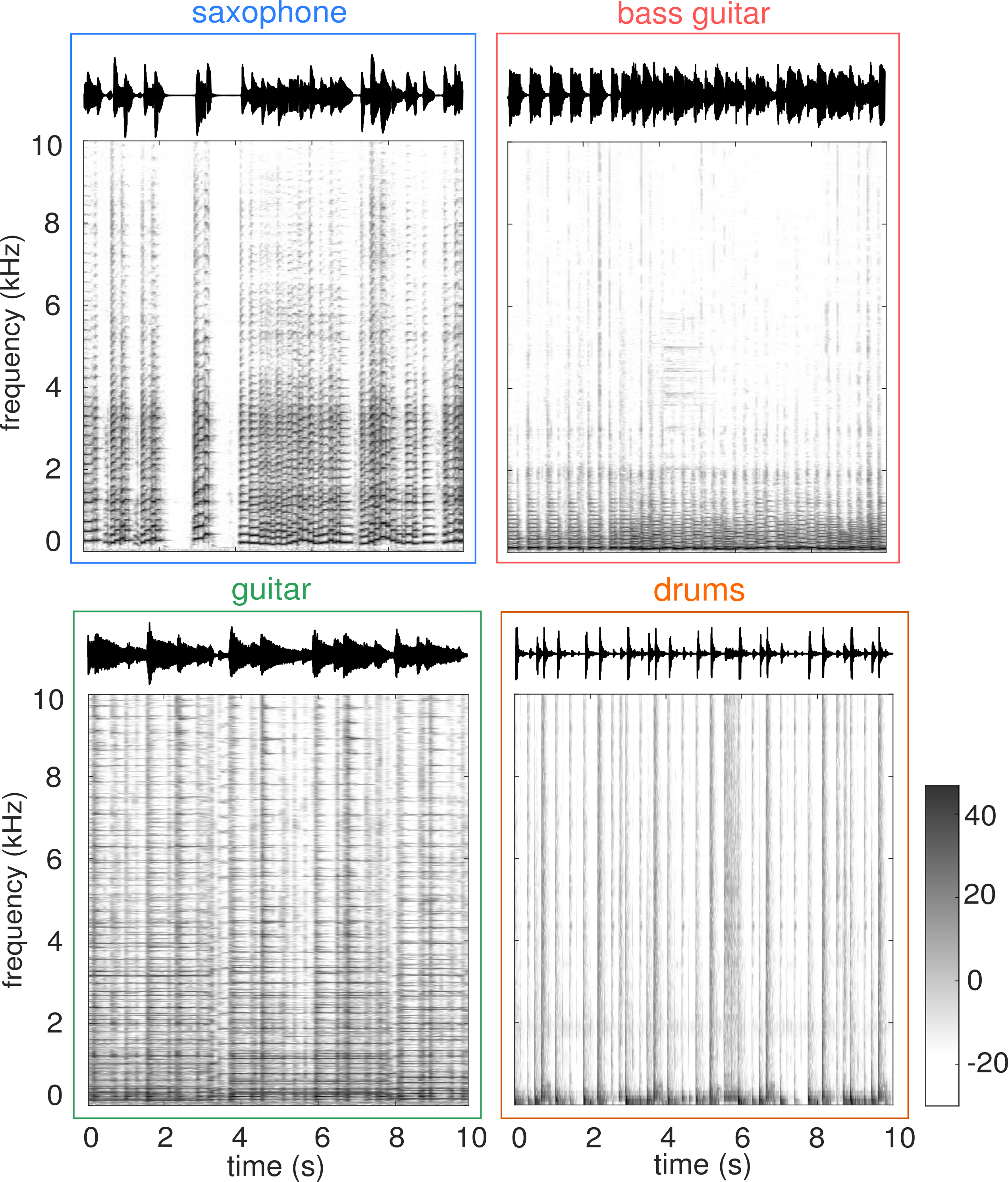
Spectrograms are frequently used as the input of machine listening systems, for the automatic retrieval of information from audio signal (e.g., voice activity detection, speech recognition, music transcription, speech emotion recognition, sound event classification), with applications in smartphones, smart speakers, robotics, domotics, smart cities, etc. A spectrogram representation is indeed much more discriminative of the constitutive elements of the sound than the raw waveform. Look for instance at the waveforms and spectrograms of the sound of different musical instruments below:

In the deep learning course, you will for instance develop a system for in-home monitoring of elderly's autonomy using spectrograms and deep neural networks.

Image, structure in the DCT domain, and compression

In a future course, we will see how the specific structure of audio signals in the time-frequency domain can be used to perform audio source separation, that is to separate different sounds from the observation of their mixture. Today, let's focus on the structure of natural images.

From 1D to 2D signal transformations

So far, we have been discussing representations of 1D signal, for instance based on the DFT or the DCT of stationary signals. We have seen that these transforms basically consist of representing a signal $\mathbf{x} \in \mathbb{R}^T$ as a linear combination of basis signals $\{\mathbf{u}_f \in \mathbb{C}^T\}_{f=0}^{F-1}$ (complex sinusoids for the DFT and cosine functions for the DCT). We have been focusing on 1D signals that represent the evolution of a quantity (e.g., the air pressure deviation) over time. However, an image is a 2D signal that represents the evolution of a quantity (e.g., light intensity) over two spatial axes, so how do we extend the 1D signal transformations to the 2D case?

The simplest approach consists of generating 2D basis signals by taking the outer product of 1D basis signals. From the basis $\{\mathbf{u}_f\}_{f=0}^{F-1}$ of $\mathbb{C}^T$ we can build a basis $\left\{\mathbf{u}_{f_1, f_2}\right\}_{f_1=0, f_2=0}^{F-1, F-1}$ of $\mathbb{C}^{T \times T}$ defined by: $$ \mathbf{u}_{f_1, f_2} = \mathbf{u}_{f_1} \mathbf{u}_{f_2}^H \in \mathbb{C}^{T \times T}, $$ or equivalently $$ \mathbf{u}_{f_1, f_2}(t_1, t_2) = \mathbf{u}_{f_1}(t_1) \mathbf{u}_{f_2}(t_2)^*, \qquad t_1, t_2 =0,...,T-1. $$

In the next cell, we compute the 2D DCT (type II) of a grayscale image and plot the image, its log-magnitude spectrum (logarithm of the absolute value of the DCT coefficients), and the image reconstruction after inverse DCT.

from utils import dct2D, idct2D
from skimage.transform import resize
from skimage.color import rgb2gray
import skimage

# get astronaut from skimage.data in grayscale
im = rgb2gray(skimage.data.astronaut())
im = resize(im, (256, 256), anti_aliasing=True)

im_DCT = dct2D(im)
im_rec = idct2D(im_DCT)

# check if the reconstructed image is nearly equal to the original image
print(np.allclose(im, im_rec))

# plot original, DCT, and reconstructed images
fig, axs = plt.subplots(1, 3, figsize=(15, 15))

im1 = axs[0].imshow(im, cmap='gray')
axs[0].set_title('original image', size=12)
axs[0].axis('off')
cax = fig.add_axes([axs[0].get_position().x1+0.01,axs[0].get_position().y0,0.02,axs[0].get_position().height])
fig.colorbar(im1, cax=cax)

im2 = axs[1].imshow(np.log10(np.abs(im_DCT)), cmap='gray')
axs[1].set_title('log of the abs. DCT coeff.', size=12)
axs[1].axis('off')
cax = fig.add_axes([axs[1].get_position().x1+0.01,axs[1].get_position().y0,0.02,axs[1].get_position().height])
fig.colorbar(im2, cax=cax)

im3 = axs[2].imshow(im_rec, cmap='gray')
axs[2].set_title('reconstructed image', size=12)
axs[2].axis('off')
cax = fig.add_axes([axs[2].get_position().x1+0.01,axs[2].get_position().y0,0.02,axs[2].get_position().height])
fig.colorbar(im3, cax=cax)

True

<matplotlib.colorbar.Colorbar at 0x7fe0d2b87ca0>

Question: How many pixels do we have in this image?

Answer: 256 x 256 = 65 536 pixels

Structure of the image in the DCT domain

We are now going to see that the image has a specific strcture in the DCT domain that it does not have in the original spatial domain, and which can be used for image compression, denoising, or more generally reconstruction of corrupted images (e.g., deblurring, inpainting, super-resolution, demosaicing, etc.) Today, we will focus on image compression.

Question: Complete the next cell to compare the histograms of the absolute value of the image and DCT coefficients. What do you observe?

im_flat = np.abs(im).flatten()

fig = plt.figure(figsize=(10,4))
ax = fig.add_subplot(111)
_ = ax.hist(im_flat, bins=100)
plt.yscale('log')
ax.set_title('Histogram of the image')

# Put you code here to plot the histogram of the DCT

Text(0.5, 1.0, 'Histogram of the image')

#### SOLUTION ####
im_flat = np.abs(im).flatten()

fig = plt.figure(figsize=(10,4))
ax = fig.add_subplot(111)
_ = ax.hist(im_flat, bins=100)
plt.yscale('log')
ax.set_title('Histogram of the image')

im_DCT_flat = np.abs(im_DCT).flatten()

fig = plt.figure(figsize=(10,4))
ax = fig.add_subplot(111)
_ = ax.hist(im_DCT_flat, bins=100)
plt.yscale('log')
ax.set_title('Histogram of the DCT')

Text(0.5, 1.0, 'Histogram of the DCT')

Answer: The DCT is sparse, most DCT coefficients are zero.

In the next cell, we plot the sorted (decreasing order) absolute values of the image and DCT coefficients (the y-axis is logarithmic).

im_flat_sort = np.flipud(np.sort(im_flat)) # sort
im_DCT_flat_sort = np.flipud(np.sort(im_DCT_flat))

fig = plt.figure(figsize=(10,5))
plt.semilogy(im_flat_sort, '-+')
plt.semilogy(im_DCT_flat_sort, '-x')
plt.title('Sorted absolute value of the image and DCT coefficients')
plt.legend(('image', 'DCT'))

<matplotlib.legend.Legend at 0x7fe0d26b2cd0>

JPEG image compression

Exercise

The JPEG compression standard leverages the sparsity of the image in the DCT domain. It works by thresholding the DCT coefficients to keep only the largest ones. That is, coefficients smaller than a given threshold are set to zero, which takes 1 bit to quantize. Complete the next cell to compare the reconstruction of the image after keeping only 1, 5, 10 and 20 % of the DCT coefficients with the largest absolute value (other coefficients will be set to zero). You will use im_DCT_flat_sort to determine the value of the threshold.

proportions = [1, 5, 10, 20] # proportion of DCT coefficients to keep

fig, axs = fig, axs = plt.subplots(1, len(proportions), figsize=(15, 15))

######### TO COMPLETE #########
n_pixels = im_DCT_flat_sort.shape[0] 

for i, prop in enumerate(proportions):
    
    thresh_index = int(prop/100*n_pixels)
    thresh_value = im_DCT_flat_sort[thresh_index]
        
    im_DCT_thresh = im_DCT.copy()
    im_DCT_thresh[np.abs(im_DCT_thresh) < thresh_value] = 0
    im_thresh = idct2D(im_DCT_thresh)
    
    axs[i].imshow(im_thresh, cmap='gray')
    axs[i].set_title('Reconstruction with ' + str(prop) + '% coeff.')

The previous image is actually a non-stationnary 2D signal. Just as we defined the STFT as a local DFT to analyze non-stationary 1D signals, we can define a local DCT to analyze non-stationary 2D images. This is what the JPEG compression standard actually does; it computes the DCT on image blocks of 8x8 pixels.

Exercise

Apply the same compression technique as in the previous cell but using a block-processing approach, i.e., computing the DCT on 8x8 blocks. Compare quantitatively and qualitatively the results with the previous global approach. You will use the Peak signal-to-noise ratio to quantify the reconstruction quality of the image.

Take-home messages

• A 1-dimensional signal can be seen as a vector in $\mathbb{R}^T$ where each element is a sample. An image is a 2D signal which can be represented as a matrix in $\mathbb{R}^{M \times N}$. If one does not care about the spatial structure of this 2D signal, it can be vectorized and seen as a 1D signal of length $MN$.

• Frequency transforms such as the DFT and the DCT correspond to the computation of the time-domain signal coordinates in a system defined by a set of basis signals. The DFT uses complex sinusoids and the DCT cosine functions:

  $$ X(f) = \langle \mathbf{x}, \mathbf{u}_f \rangle = \mathbf{u}_f^H \mathbf{x}, \qquad f \in \{0,...,F-1\}. $$

  The inverse transform simply expresses that the signal can be synthesized as a linear combination of the basis signals:

  $$ \mathbf{x} = \sum\limits_{f=0}^{F-1} X(f) \mathbf{u}_f = \sum\limits_{f=0}^{F-1} \langle \mathbf{x}, \mathbf{u}_f \rangle \mathbf{u}_f. $$

  The DFT or DCT coefficient $\hat{x}(f)$ encodes the contribution of the basis signal $\mathbf{u}_f$ in the original signal $\mathbf{x}$. We have seen that by simply zeroing coefficients at specific frequencies we can cancel out some components of the signal. This is called filtering, an example of signal transformation.

• Frequency transforms can be extended to 2D signals by building a family of 2D basis signals defined as the outer product of the 1D basis signals.

• The DFT and the DCT are only appropriate for stationary signals. For non-stationary signals, e.g., when the frequency characteristics of the signal vary with time or space, we have to use a local transform that focuses on local properties of the signal. A local transform can be built by windowing the signal before computing a standard transform such as the DFT or DCT. For temporal signals windowing means focusing on a temporal windows, for images it means focusing on a small patch of the image.

  The STFT is a time-frequency transform defined by computing the DFT on short overlapping frames of the signal. Just as the DFT and DCT, the STFT can be interpreted as decomposing the signals over a set of basis signals, which are called time-frequency atoms and that simply correspond to the DFT complex sinusoids localized in time.

• Many real-life applications build upon algorithms that process signals, sounds, images in a transformed domain (e.g., frequency or time-frequency domains). This is because natural signals and images exhibit specific properties in these transform domains, which can be leveraged for different signal processing tasks such as signal transformation, compression, denoising, or reconstruction. For instance, we have seen today that images are sparse in the DCT domain, a property that is at the basis of the JPEG compression standard.

To conclude, let us stress that without signal processing, the phase vocoder would not exist, the autotune would not exist, and Jul) would not have become in 2020 the best-selling artist in the history of French rap.

Appendices

Discrete-time Fourier transform

Definition

Let $x(t) \in \mathbb{R}$ be a signal defined in the time domain $t \in \mathbb{Z}$ such that $\sum\limits_{t \in \mathbb{Z}} |x(t)| < \infty$.

The discrete-time Fourier transform is defined by

$$ \hat{x}(\nu) = \sum\limits_{t \in \mathbb{Z}} x(t) e^{-j 2 \pi \nu t}, $$

where $\nu$ is called the normalized frequency.

By definition, the DTFT is periodic with period 1:

$$\hat{x}(\nu + 1) = \sum\limits_{t \in \mathbb{Z}} x(t) e^{-j 2 \pi (\nu +1) t} = \sum\limits_{t \in \mathbb{Z}} x(t) e^{-j 2 \pi \nu t} e^{-j 2 \pi t} = \sum\limits_{t \in \mathbb{Z}} x(t) e^{-j 2 \pi \nu t} = \hat{x}(\nu). $$

We thus limit its representation to the interval $\nu \in [-0.5, 0.5[$ or $\nu \in [0, 1[$.

The inverse discrete-time Fourier transform is defined by:

$$ x(t) = \int_{-1/2}^{1/2} \hat{x}(\nu) e^{+j 2 \pi \nu t} d\nu.$$

Properties of the DTFT (time domain $\leftrightarrow$ frequency domain)

• Linearity: $a x(t) + by(t)$ $\leftrightarrow$ $a\hat{x}(\nu) + b\tilde{y}(\nu)$
• Time shift: $x(t-t_0)$ $\leftrightarrow$ $\hat{x}(\nu) e^{-j 2 \pi \nu t_0}$
• Frequency shift: $x(t) e^{j 2 pi \nu_0 t}$ $\leftrightarrow$ $\hat{x}(\nu-\nu_0)$
• Convolution: $ [x \star y] (t) = \sum\limits_{k \in \mathbb{Z}} x(k) y(t-k) $ $\leftrightarrow$ $\hat{x}(\nu) \tilde{y}(\nu)$
• Hermitian symmetry: $ x(t) \in \mathbb{R}$ $\leftrightarrow$ $\hat{x}(\nu) = \hat{x}^{*}(1-\nu) $

Real-world signals

In practice, we acquire signals during a limited period of time and using sensors with limited dynamics. The consequence is that the signals are of finite length, amplitude, and energy. We therefore always have:

• $ x(t) \neq 0$ only for $t \in \{0,...,T-1 \}$, this set being called the time support of the signal;

• $ \sum\limits_{t \in \mathbb{Z}} |x(t)| = \sum\limits_{t=0}^{T-1} |x(t)| < \infty$.

We could therefore also represent this signal as a vector $\mathbf{x} \in \mathbb{R}^T$, where the entry of index $t \in \{0,...,T-1 \}$ contains the sample $x(t)$.

Sampling the DTFT gives the DFT

In practice, we also work with a finite subset of frequencies. We fix a number of frequencies $F \in \mathbb{N}$ and define

$$ \nu_f = \frac{f}{F} \in [0, 1[, \qquad f \in \{0,...,F-1\}.$$

By sampling the DTFT of a signal of finite length $T$ we obtain the discrete Fourier transform (DFT):

$$ \hat{x}(\nu_f) = \sum\limits_{t \in \mathbb{Z}} x(t) e^{-j 2 \pi \frac{f}{F} t} = \sum\limits_{t=0}^{T-1} x(t) e^{-j 2 \pi \frac{f}{F} t} = X(f). $$

A consequence of this sampling is the periodization of the time-domain signal, which is also why we need to assume a finite-support signal when defining the DFT.

DTFT and DFT of simple signals, precision and resolution

Constant signal

We consider the following finite-length constant signal defined for $t \in \mathbb{Z}$ by

$$ x(t) = \begin{cases} 1 &\text{if } t \in \{0,...,T-1\} \\ 0 &\text{otherwise}, \end{cases} $$

Its DTFT is given by:

$$ \hat{x}(\nu) = \frac{\sin(\pi \nu t)}{\sin(\pi \nu)} e^{-j\pi\nu(T-1)}. $$

In the next cell, we plot the magnitude spectrum of this signal computed with the DTFT and DFT, for the different lengths. We observe a spectrum with the shape of a sine cardinal, and the presence of a principal lobe of width $2/T$.

We can conclude that the shorter the time-domain signal, the larger the pricipal lobe, the lower the resolution.

T_vec = np.array([16, 32, 64])
    
plt.subplots(3,2, figsize=(15,10))

nu0 = 0.1
nu1 = 0.13
F = 128
f = np.arange(F)
T_max = np.max(T_vec)

for ind, T in enumerate(T_vec):

    t = np.arange(T_max)

    ## Constant
    x = np.zeros(T_max)
    x[:T] = 1

    ## Sinusoid
    # x = np.sin(2*np.pi*nu0*t)
    # x[T:] = 0

    ## Sum of sinusoids
    # x = .5*np.sin(2*np.pi*nu0*t) + .5*np.sin(2*np.pi*nu1*t)
    # x[T:] = 0

    x_dtft = np.fft.fft(x, F)
    x_dft = np.fft.fft(x, T)

    plt.subplot(3,2,ind*2+1)
    plt.plot(t, x, '-')
    plt.plot(t, x, 'o', fillstyle='none')
    plt.xlim(0,T_max)
    plt.ylim(-1.1,1.1)

    if ind==0:
        plt.title('Finite-length signal')

    if ind==2:
        plt.xlabel('time')

    plt.yticks(np.array([0,1]), np.array([0,1]))

    plt.subplot(3,2,ind*2+2)
    plt.plot(f/F, np.abs(x_dtft), '-')
    plt.plot(np.arange(T)/T, np.abs(x_dft), 'o', fillstyle='none')

    if ind==0:
        plt.title('Magnitude spectra')
        plt.legend([r'DTFT $\hat{x}(\nu)$', r'DFT $\hat{x}(f) = \hat{x}(f/T)$'], loc='upper right', fontsize=16)

    if ind==2:
        plt.xlabel('frequency')

Sinusoid

We now consider the following finite-length sinusoid defined for $t \in \mathbb{Z}$ by

$$ x(t) = \begin{cases} \sin (2 \pi \nu_0 t) &\text{if } t \in \{0,...,T-1\} \\ 0 &\text{otherwise}, \end{cases} $$

where $\nu_0 = 0.1$ and $T \in \{16,32,64\}$.

In the previous code cell, uncomment the appropriate lines (CTRL + '/') to plot the magnitude spectrum of this sinusoid, for the different lengths. You should observe two principal lobes centered around $\nu_0$ and $- \nu_0$. The same principle applies regarding the resolution: the more periods we observe, the "more certain" we are about the pure tone frequency.

Note that the blue curve is actually an interpolation of the DFT of order $F = 128$. Increasing the order of the DFT simple increases the precision, i.e. the number of points used to sample the DTFT, it does not change the resolution.

Sum of sinusoids

We now consider the following sum of two sinusoids with close normalized frequencies:

$$ \forall t \in \mathbb{Z}, \qquad x(t) = \begin{cases} \sin (2 \pi \nu_0 t) + \sin (2 \pi \nu_1 t) &\text{if } t \in \{0,...,T-1\} \\ 0 &\text{otherwise} \end{cases} $$

where

• $\nu_0 = 0.1$
• $\nu_1 = 0.13$
• $T \in \{16,32,64\}$

In the previous code cell, uncomment the appropriate lines (CTRL + '/') to plot the magnitude spectrum of this signal, for the different lengths. You should observe that for $T=16$, the resolution is not sufficient to separate the two frequencies.

References

Parts of this notebook were inspired/adapted by/from the following resources:

• Mathematical Tools for Data Science course at NYU by Carlos Fernandez-Granda.
• Signal processing course at Ecole Polytechnique by Rémi Flamary.